
We often use recurrent neural network architectures for use cases such as streaming, where we make a new prediction each time new information arrives. It’s common to give it a long context each time, which repeats work and is therefore computationally wasteful. In this blog post, I will illustrate multiple ways to perform inference step by step using recurrent architectures by remembering the states and therefore removing the need to unnecessarily compute the same steps over and over. My post Creating a custom training loop in tensorflow gives a quick start on the Keras functional API which I use for the main code snippets.
Context
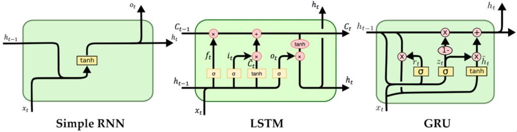
Recurrent Neural Networks (RNNs) are a popular type of neural network which specialises in time series data. Just like our brains are able to interpret a series of images as a movie or a bunch of words as a sentence, so a recurrent neural network is able to remember the past inputs, which affect its output for future inputs. It does this by maintaining a hidden state which is fed forward to the next iteration in a recurrent fashion. The unit that takes the previous state and input as inputs and returns the context is called a cell.
To improve this basic principle, architectures such as the LSTM (Long Short-Term Memory) improve on the vanilla RNN cell by including a separate cell state and special gates that “remember” and “forget” to and from the cell state. This greatly improves the ability of these networks to remember long sequences. This post will focus on the LSTM cell due to the extra complexity from the second state but can be easily adapted to the other main recurrent architecture used, the GRU cell.
The wasteful approach
The wasteful approach provides the entire context for each time step. To predict timestep i, the model receives inputs [0..i] as context. Since the hidden state after time step k, 0<=k<i is deterministically the same, repeating the computation is unnecessary.
First, we need to define imports, fix the seed, set the parameters for the models and generate a random input that we will reuse with all the models:
# Imports
import tensorflow as tf
import tensorflow.keras.layers as L
import matplotlib.pyplot as plt
from time import perf_counter

# Fix the seed so it always generates the same X and weights
tf.random.set_seed(0)

# Define parameters
batch_size = 10
seq_length = 200
features = 4
lstm_1_units = 100
lstm_2_units = 200

# Generate a random input for all models
X = tf.random.uniform((batch_size, seq_length, features))
The “classic” way. A standard model, as expected.
input1 = L.Input((None, 4))
lstm1_1 = L.LSTM(lstm_1_units, return_sequences=True)
lstm1_1_o = lstm1_1(input1)
lstm2_1 = L.LSTM(lstm_2_units)
lstm2_1_o = lstm2_1(lstm1_1_o)
output_dense_1 = L.Dense(1, activation="sigmoid")
output1 = output_dense_1(lstm2_1_o)
model1 = tf.keras.Model(inputs=input1, outputs=output1)
start1 = perf_counter()
classic_results = []
for i in range(1, len(X[0])):
result_batch = model1.predict(X[:, 0:i, :])
classic_results.append(result_batch[0][0])
stop1 = perf_counter()
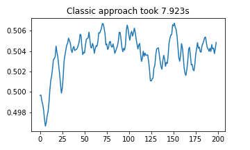
plt.plot(classic_results)
plt.title(f"Classic approach took {(stop1 - start1):.03f}s")
plt.show()
To improve the performance, we often restrict the context by only providing [i-B..i]. This is significantly better computationally, though it also repeats most operations, and restricts the model from having access to as much of the data as potentially useful.
The stateful model
Keras offers “stateful=True” for LSTM layers which maintain state automatically.
This is good if you always have the same sequence order in the batch, e.g.,
- you are streaming live data and you are always appending to the same sequence
- you want to evaluate a long sequence without keeping the entire thing in memory
It needs to know its batch size to be stateful, therefore it is specified for Input
input2 = L.Input((None, 4), batch_size=batch_size)

lstm1_2 = L.LSTM(lstm_1_units, return_sequences=True, stateful=True)
lstm1_2_o = lstm1_2(input2)

lstm2_2 = L.LSTM(lstm_2_units, stateful=True)
lstm2_2_o = lstm2_2(lstm1_2_o)

output_dense_2 = L.Dense(1, activation="sigmoid")
output2 = output_dense_2(lstm2_2_o)

model2 = tf.keras.Model(inputs=input2, outputs=output2)

# Copy the weights from the first model
lstm1_2.set_weights(lstm1_1.get_weights())
lstm2_2.set_weights(lstm2_1.get_weights())
output_dense_2.set_weights(output_dense_1.get_weights())

start2 = perf_counter()

stateful_results = []
for i in range(len(X[0]) - 1):
    # Since it's stateful, we can get each time step one by one
    # entire batch, from i->i+1, entire feature list
    result_batch = model2.predict(X[:, i : i + 1, :])
    stateful_results.append(result_batch[0][0])

stop2 = perf_counter()

plt.plot(stateful_results)
plt.title(f"Stateful model took {(stop2 - start2):.03f}s")
plt.show()

Step by step inference using the functional API
Maybe items in the batch change, or are not always present
Manually managing the state is useful as it allows some items in the batch to continue processing
The stateful approach only allows reset_states(), but that clears all of them
using the functional model we can accept multiple inputs which we pass as c,h
This model takes as inputs the c,h for lstm1, lstm2
returns new c,h for lstm1, lstm2
An input for each c,h
And returns each c,h
Management of them can then be done in the prediction loop as required or saved for later.
input3 = L.Input((None, features))
lstm1_3_c_input = L.Input((lstm_1_units,))
lstm1_3_h_input = L.Input((lstm_1_units,))
lstm2_3_c_input = L.Input((lstm_2_units,))
lstm2_3_h_input = L.Input((lstm_2_units,))
lstm1_3 = L.LSTM(lstm_1_units, return_sequences=True, return_state=True)
lstm1_3_o, lstm1_3_h, lstm1_3_c = lstm1_3(
input3, initial_state=[lstm1_3_h_input, lstm1_3_c_input]
)
lstm2_3 = L.LSTM(lstm_2_units, return_state=True)
lstm2_3_o, lstm2_3_h, lstm2_3_c = lstm2_3(
lstm1_3_o, initial_state=[lstm2_3_h_input, lstm2_3_c_input]
)
output_dense_3 = L.Dense(1, activation="sigmoid")
output3 = output_dense_3(lstm2_3_o)
model4 = tf.keras.Model(
inputs={
"input": input3,
"lstm1_h": lstm1_3_h_input,
"lstm1_c": lstm1_3_c_input,
"lstm2_h": lstm2_3_h_input,
"lstm2_c": lstm2_3_c_input,
},
outputs={
"output": output3,
"lstm1_h": lstm1_3_h,
"lstm1_c": lstm1_3_c,
"lstm2_h": lstm2_3_h,
"lstm2_c": lstm2_3_c,
},
)
lstm1_3.set_weights(lstm1_1.get_weights())
lstm2_3.set_weights(lstm2_1.get_weights())
output_dense_3.set_weights(output_dense_1.get_weights())
# Initialise cell hidden states, default zeros
lstm1_3_h_val = tf.zeros((batch_size, lstm_1_units))
lstm1_3_c_val = tf.zeros((batch_size, lstm_1_units))
lstm2_3_h_val = tf.zeros((batch_size, lstm_2_units))
lstm2_3_c_val = tf.zeros((batch_size, lstm_2_units))
start3 = perf_counter()
manual_func_results = []
for i in range(len(X[0]) - 1):
ts_res = model4.predict(
{
"input": X[:, i : i + 1, :],
"lstm1_h": lstm1_3_h_val,
"lstm1_c": lstm1_3_c_val,
"lstm2_h": lstm2_3_h_val,
"lstm2_c": lstm2_3_c_val,
}
)
manual_func_results.append(ts_res["output"][0][0])
lstm1_3_h_val = ts_res["lstm1_h"]
lstm1_3_c_val = ts_res["lstm1_c"]
lstm2_3_h_val = ts_res["lstm2_h"]
lstm2_3_c_val = ts_res["lstm2_c"]
stop3 = perf_counter()
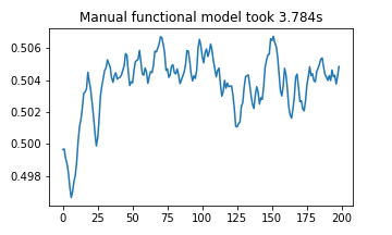
plt.plot(manual_func_results)
plt.title(f"Manual functional model took {(stop3 - start3):.03f}s")
plt.show()
Step by step inference using the subclassed model
class SubclassedModel(tf.keras.Model):
    def __init__(self):
        super().__init__()
        self.lstm1 = L.LSTM(lstm_1_units, return_sequences=True, return_state=True)
        self.lstm2 = L.LSTM(lstm_2_units, return_state=True)
        self.output_dense = L.Dense(1, activation="sigmoid")

    def call(self, inputs):
        lstm1_o, lstm1_h, lstm1_c = self.lstm1(
            inputs["input"], initial_state=[inputs["lstm1_h"], inputs["lstm1_c"]]
        )
        lstm2_o, lstm2_h, lstm2_c = self.lstm2(
            lstm1_o, initial_state=[inputs["lstm2_h"], inputs["lstm2_c"]]
        )
        output_dense = self.output_dense(lstm2_o)
        return {
            "output": output_dense,
            "lstm1_h": lstm1_h,
            "lstm1_c": lstm1_c,
            "lstm2_h": lstm2_h,
            "lstm2_c": lstm2_c,
        }


model4 = SubclassedModel()
model4.build(
    input_shape={
        "input": (batch_size, None, features),
        "lstm1_h": (batch_size, lstm_1_units),
        "lstm1_c": (batch_size, lstm_1_units),
        "lstm2_h": (batch_size, lstm_2_units),
        "lstm2_c": (batch_size, lstm_2_units),
    }
)

model4.lstm1.set_weights(lstm1_1.get_weights())
model4.lstm2.set_weights(lstm2_1.get_weights())
model4.output_dense.set_weights(output_dense_1.get_weights())


lstm1_4_h_val = tf.zeros((batch_size, lstm_1_units))
lstm1_4_c_val = tf.zeros((batch_size, lstm_1_units))
lstm2_4_h_val = tf.zeros((batch_size, lstm_2_units))
lstm2_4_c_val = tf.zeros((batch_size, lstm_2_units))

state = {
    "lstm1_h": lstm1_4_h_val,
    "lstm1_c": lstm1_4_c_val,
    "lstm2_h": lstm2_4_h_val,
    "lstm2_c": lstm2_4_c_val,
}

start4 = perf_counter()
manual_subcl_results = []
for i in range(len(X[0]) - 1):
    state["input"] = X[:, i : i + 1, :]
    state = model4.predict(state)
    manual_subcl_results.append(state["output"][0][0])
stop4 = perf_counter()

plt.plot(manual_subcl_results)
plt.title(f"Subclassed model took {(stop4 - start4):.03f}")
plt.show()

Ensuring all outputs were identical
assert tf.reduce_all(classic_results == stateful_results)
assert tf.reduce_all(stateful_results == manual_func_results)
assert tf.reduce_all(manual_func_results == manual_subcl_results)
Conclusion
Recurrent architectures are known for being slow, and it’s important to notice the speedup obtained even with such a small model. Knowing how to manually manage recurrent hidden states improves the performance of machine learning models used for streaming or deployed in stateless containers
Jupyter notebook here