
Dimensionality reduction is useful in compressing the representation of your data. In my last post, how not to reduce dimensionality for clustering, I show a neural network that reduces the 784 dimensions of the MNIST dataset into 3, which are constrained by the k-means algorithm to capture the essence of the data. This week we’ll be looking to reduce the dimensionality of MNIST using autoencoders since it is a more common approach.
Autoencoders are a type of neural network which constrain the output to be the same as the input. The information passes through a bottleneck of low dimensionality. This has the effect of letting the network learn how to embed all the relevant information into a smaller representation.
The model
Let’s go through the code in order to see how it’s done. As usual, we start with the imports and some definitions. Check out my shapes posts if you’re confused about reshaping.
import tensorflow as tf
import matplotlib.pyplot as plt
from mpl_toolkits.mplot3d import Axes3D
import matplotlib.patches as mpatches

# colour list for plotting
colours = ['#00FA9A','#FFFF00','#2F4F4F','#8B0000','#FF4500','#2E8B57','#6A5ACD','#FF00FF','#A9A9A9','#0000FF']

# number of features for the encoded number
encoded_dim = 3

# load MNIST data
(x_train, y_train), (x_test, y_test) = tf.keras.datasets.mnist.load_data()

# scale between 0 and 1
X = tf.constant(x_train/255.0)

# reshape since we're feeding it into a dense layer
X = tf.reshape(X, (-1, 28*28))
The autoencoder consists of two parts: the encoder and the decoder. We use the decoder to handle dimensionality reduction and the decoder to recreate the original data. We’ll build a functional model in order to be able to split the model into pieces.
# First the encoder
enc_input = tf.keras.layers.Input(shape=(28*28,))
enc_inner = tf.keras.layers.Dense(28*28, activation="sigmoid")(enc_input)
enc_inner = tf.keras.layers.Dense(64, activation="sigmoid")(enc_inner)
enc_inner = tf.keras.layers.Dense(32, activation="sigmoid")(enc_inner)
enc_output = tf.keras.layers.Dense(encoded_dim, activation="sigmoid")(enc_inner)

# Then the decoder
dec_inner = tf.keras.layers.Dense(32, activation="sigmoid")(enc_output)
dec_inner = tf.keras.layers.Dense(64, activation="sigmoid")(dec_inner)
dec_output = tf.keras.layers.Dense(28*28, activation="sigmoid")(dec_inner)

# Define the whole autoencoder from enc_input to dec_output
autoencoder = tf.keras.Model(inputs=enc_input, outputs=dec_output)

# The encoder stops at enc_output
encoder = tf.keras.backend.function(enc_input, enc_output)

# compile the model so we penalise based on mean squared error between pixels
autoencoder.compile(optimizer="adam", loss="mse")
I like using EarlyStopping so I don’t waste time training. It works by stopping training if the model accuracy does not improve over more than 10 epochs. We let it fit for a maximum of 500 epochs, but in practice, it stops before 100. Notice how we fit using X both as input and labels.
es = tf.keras.callbacks.EarlyStopping(monitor='loss', patience=10, min_delta=0.0005)
autoencoder.fit(X, X, epochs=500, callbacks=[es])
How Does it perform?
We can plot both the original and the autoencoded images to see how well the model performs. The higher the encoded dimension, the more accurate the result. Let’s see how encoding into 3 dimensions compares to 10 dimensions.
# Plot autoencoder outputs compared to inputs
def plot_examples(autoencoder, X):
    fig = plt.figure(figsize=(5,2*len(X)))
    output = autoencoder(X)
    X = tf.reshape(X, (-1, 28, 28))
    output = tf.reshape(output, (-1, 28, 28))

    for j,(i,o) in enumerate(zip(X, output)):
        ax = fig.add_subplot(len(X), 2, 2*j+1)
        ax.imshow(i)
        ax = fig.add_subplot(len(X), 2, 2*j+2)
        ax.imshow(o)

plot_examples(autoencoder, X[:9])
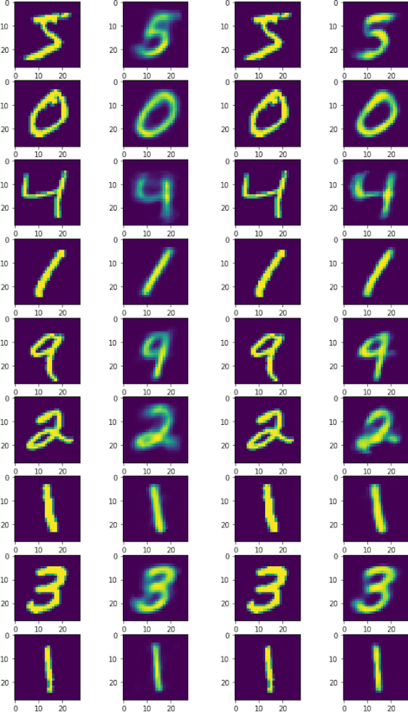
Using 10 dimensions yields more detailed outputs, but the 3 dimension model isn’t bad at all. However, The bonus to using 3 dimensions is being able to easily plot the intermediate representation as a 3D plot.
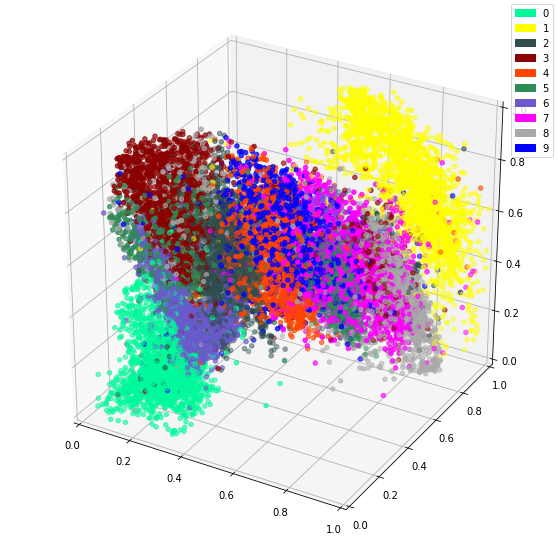
It is impressive seeing how dots representing the same digit continue to be close together even in 3 dimensions. I imagine there will be little surprise about the theme of my next post.
Thanks for reading! I hope this post was interesting since autoencoders are a cool type of neural network. As an example, we can reduce dimensionality using autoencoders to compress data or to extract important features.
Pingback: Using Machine Learning to Compromise between names - Felix Gravila