Clustering on encoding

In the past, I’ve covered how to implement k-means and how to cluster MNIST directly. Then I showed a bad way to reduce dimensionality for clustering. Finally, we used an autoencoder on MNIST. In this post, we’ll join everything together by performing clustering on the encoding and see how it performs.

In the previous post, we’ve used an autoencoder to encode the MNIST dataset. By constraining all 784 dimensions of the images into the 3 of the bottleneck, we hoped similar digits would be clustered together. We confirmed this since we could see a clear clustering when colour coding by digit.

It follows that a great idea would be to cluster this encoding as we hope the important features were already extracted. Remember that the goal of this exercise is unsupervised learning. The neural network is able to extract features combining multiple pixels, therefore increasing its power.

Autoencoder again

The first part of the code forms the same autoencoder. First some definitions:

import tensorflow as tf
import matplotlib.pyplot as plt
from mpl_toolkits.mplot3d import Axes3D
import matplotlib.patches as mpatches
import numpy as np

# colour list for plotting
colours = ['#00FA9A','#FFFF00','#2F4F4F','#8B0000','#FF4500','#2E8B57','#6A5ACD','#FF00FF','#A9A9A9','#0000FF']

# number of features for the encoded number
encoded_dim = 3

# load MNIST data
(x_train, y_train), (x_test, y_test) = tf.keras.datasets.mnist.load_data()

# scale between 0 and 1
X = tf.constant(x_train/255.0)

# reshape since we're feeding it into a dense layer
X = tf.reshape(X, (-1, 28*28))

We redefine the model the same way. It can be trained by compiling and fitting like previous or just load the previous model from the weights file. The model can be loaded completely from the h5 file without having to redefine it. Since we split the autoencoder, we redefine it so we have access to the layers using which we build our encoder and decoder.

# Define the model again so we can load the weights from last time and split into encoder/decoder

# First the encoder
enc_input = tf.keras.layers.Input(shape=(28*28,), name="enc_input")
enc_inner = tf.keras.layers.Dense(28*28, activation="sigmoid", name="enc_dense_1")(enc_input)
enc_inner = tf.keras.layers.Dense(64, activation="sigmoid", name="enc_dense_2")(enc_inner)
enc_inner = tf.keras.layers.Dense(32, activation="sigmoid", name="enc_dense_3")(enc_inner)
enc_output = tf.keras.layers.Dense(encoded_dim, activation="sigmoid", name="enc_output")(enc_inner)

# Then the decoder
dec_inner = tf.keras.layers.Dense(32, activation="sigmoid", name="dec_dense_1")(enc_output)
dec_inner = tf.keras.layers.Dense(64, activation="sigmoid", name="dec_dense_2")(dec_inner)
dec_output = tf.keras.layers.Dense(28*28, activation="sigmoid", name="dec_output")(dec_inner)

# Define the whole autoencoder from enc_input to dec_output
autoencoder = tf.keras.Model(inputs=enc_input, outputs=dec_output, name="autoencoder")

# The encoder stops at enc_output
encoder = tf.keras.backend.function(enc_input, enc_output)
# decoder from enc_output to dec_output
decoder = tf.keras.backend.function(enc_output, dec_output)

autoencoder.load_weights(f"autoenc_{encoded_dim}.h5")

To have saved the model in the last post, simply add the following after training it:

autoencoder.save(f"autoenc_{encoded_dim}.h5")

K-means

We can use the K-means code from the clustering MNIST post.

# define number of clusters
clusters_n = 10

pred = encoder(X)

centroids = tf.slice(tf.compat.v1.random_shuffle(pred), [0, 0], [clusters_n, -1])
points_expanded = tf.expand_dims(pred, 0)

@tf.function
def update_centroids(points_expanded, centroids):
    centroids_expanded = tf.expand_dims(centroids, 1)
    distances = tf.subtract(centroids_expanded, points_expanded)
    distances = tf.square(distances)
    distances = tf.reduce_sum(distances, 2)
    assignments = tf.argmin(distances, 0)

    means = []
    for c in range(clusters_n):
        eq_eq = tf.equal(assignments, c)
        where_eq = tf.where(eq_eq)
        ruc = tf.reshape(where_eq, [1,-1])
        ruc = tf.gather(pred, ruc)

        ruc = tf.reduce_mean(ruc, axis=[1])
        means.append(ruc)
        new_centroids = tf.concat(means, 0)

    return new_centroids, assignments

old_centroids = centroids
while True:
    centroids, assignments = update_centroids(points_expanded, centroids)
    if tf.reduce_all(centroids == old_centroids):
        break
    old_centroids = centroids


# classify points using trained centroids
# same code as for update_centroids, but only returns the argmin
def get_assignments(centroids, y_pred):
    points_expanded = tf.expand_dims(y_pred, 0)
    centroids_expanded = tf.expand_dims(centroids, 1)
    distances = tf.subtract(centroids_expanded, points_expanded)
    distances = tf.square(distances)
    distances = tf.reduce_sum(distances, 2)
    assignments = tf.argmin(distances, 0)
    return assignments

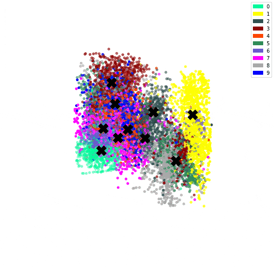
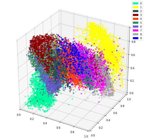
We can then plot the representation with the centroids.

# Plot the encoded representations and the centroids
if encoded_dim == 3:
    num_to_plot = 10000
    pred = encoder(X[:num_to_plot])
    fig = plt.figure(figsize=(10,10))
    ax = fig.add_subplot(111, projection='3d')

    ax.scatter(pred[:,0], pred[:,1], pred[:,2], zorder=1, color=[colours[y] for y in y_train[:num_to_plot]])
    ax.plot(centroids[:, 0], centroids[:, 1], centroids[:, 2], "kX", markersize=20, zorder=1000)
    mpc = []
    for i in range(10):
        mpatch = mpatches.Patch(color=colours[i], label=i)
        mpc.append(mpatch)
    plt.legend(handles=mpc)

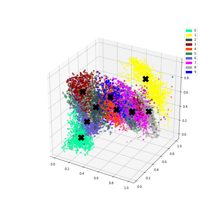
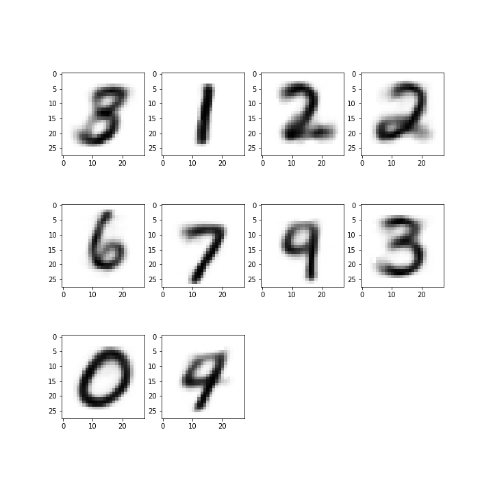
Since we have both an encoder and decoder, and the centroids are in the feature space of the encoding, we can use the decoder to see what the centroids look like.

# Get reconstructed numbers for centroids
reconst = decoder(centroids)

fig = plt.figure(figsize=(10, 10))
for i, c in enumerate(reconst):
    ax = fig.add_subplot(3, 4, i+1)
    plt.imshow(tf.reshape(c, (28, 28)), cmap="gray_r")

Finally, let’s have a look at the purity

def calc_purity(labels, assignments):
    d = np.zeros((clusters_n, clusters_n), dtype="int32")
    for l, a in zip(labels, assignments):
        d[a][l] += 1

    purity_per_class = d.max(1)/d.sum(1)
    # some are NaN
    purity_per_class = purity_per_class[~np.isnan(purity_per_class)]
    return np.mean(purity_per_class)

# Perform prediction on the dataset to get the intermediate representation
predict_batch_size = 10000
predict_count = len(X)

m = []
for i in range(0, predict_count, predict_batch_size):
    m.append(encoder(X[i:i+predict_batch_size]))
res = tf.concat(m, 0)

assignments = get_assignments(centroids, res)

calc_purity(y_train[:predict_count], assignments)

0.6988619101877526

Already better than the 0.62 obtained by directly clustering on the pixels.

Conclusion

I hope this post illustrated the power of clustering on the encoding by using an autoencoder. Beside being able to use the power of a neural network to extract complex features, the decoder enables us to directly reconstruct the centroids, giving us a better intuition of what they are doing, which can increase trust in the model.