This is the beginning of a series in which we’ll explore ways to perform clustering. In particular, we’ll perform clustering on the MNIST dataset, since it’s a dataset of high dimensionality which is easy to understand. In my previous post, ‘How to implement the K-means algorithm in Tensorflow‘, I explain the code of Sergey Kovalev, Sergei Sintsov, and Alex Khizhniak line by line, and expand it a bit. Understanding K-means will be important for this series, but skipping the implementation is fine.
Clustering is a type of machine learning that finds patterns in data without being told what to do. It’s very useful in situations where we want to separate a dataset of which we do not know much. The MNIST dataset is great for illustrating the point: it consists of 70,000 images of 28×28 pixels depicting handwritten digits.
MNIST is a labeled dataset. For each image, we get a label that tells us what the depicted number is supposed to be. Using this information we could easily create a supervised learning model such as a CNN, and reach very high accuracies. For the purposes of this series let’s assume we do not have access to the labels. Instead of 28×28 pixels, let’s imagine they are 784 individual sensor readings. Is it possible to get a machine learning model to designate a class to each number without any labels?
K-means does exactly this. The only parameter it requires, K, tells it how many classes to find. It is a simple algorithm with an easy to understand loop. First, it assigns K random centroids (items in the feature space of the original data). Then, until it converges, it assigns the closest centroid to each data point, then moves the centroid to the mean of all assigned data points. K-means always converges, though not necessarily to a global minimum. Make sure to read my other post for a rundown of the algorithm, since I’ll be skipping over the details in this one.
Direct implementation on the feature space
Let’s adapt the algorithm to do some clustering on MNIST. As a first example to show its problems, let’s directly cluster on the original feature space. For us this means 784 dimensions. The only thing we need to do is flatten the images. If shapes confuse you, I have a few posts on that (intro and closer look).
import tensorflow as tf import numpy as np import matplotlib.pyplot as plt import random # we want to split into 10 clusters, one for each digit clusters_n = 10 # load MNIST data (x_train, y_train), (x_test, y_test) = tf.keras.datasets.mnist.load_data() # flatten the digits into arrays of 784 pixels flattened = x_train.reshape(-1, 28*28)/255.0 flattened = tf.constant(flattened)
We now have data exactly as we needed it in the last post. Let’s run the same algorithm.
centroids = tf.slice(tf.compat.v1.random_shuffle(flattened), [0, 0], [clusters_n, -1])
points_expanded = tf.expand_dims(flattened, 0)

@tf.function
def update_centroids(points_expanded, centroids):
  centroids_expanded = tf.expand_dims(centroids, 1)
  distances = tf.subtract(centroids_expanded, points_expanded)
  distances = tf.square(distances)
  distances = tf.reduce_sum(distances, 2)
  assignments = tf.argmin(distances, 0)

  means = []
  for c in range(clusters_n):
    eq_eq = tf.equal(assignments, c)
    where_eq = tf.where(eq_eq)
    ruc = tf.reshape(where_eq, [1,-1])
    ruc = tf.gather(flattened, ruc)

    ruc = tf.reduce_mean(ruc, axis=[1])
    means.append(ruc)
    new_centroids = tf.concat(means, 0)

  return new_centroids, assignments

old_centroids = centroids
while True:
  centroids, assignments = update_centroids(points_expanded, centroids)
  if tf.reduce_all(centroids == old_centroids):
    break
  old_centroids = centroids
We now have both our centroids and an assignment for each image. We can make a simple function to show us a few example pictures from each class. Since the algorithm had no idea what is what, the classes do not necessarily match the number, unless your random picks were very lucky.
def examples_of(number, rows=5, cols=5):
fig = plt.figure(figsize=(7,7))
ax = []
i=0
while len(ax) < rows*cols:
if assignments[i] == number:
ax.append(fig.add_subplot(rows, cols, len(ax)+1))
plt.imshow(x_train[i], cmap="gray_r")
i+=1
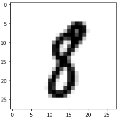
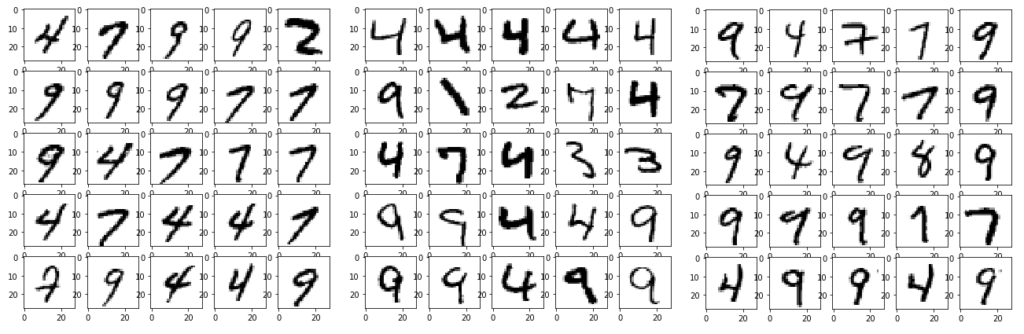
examples_of(8)
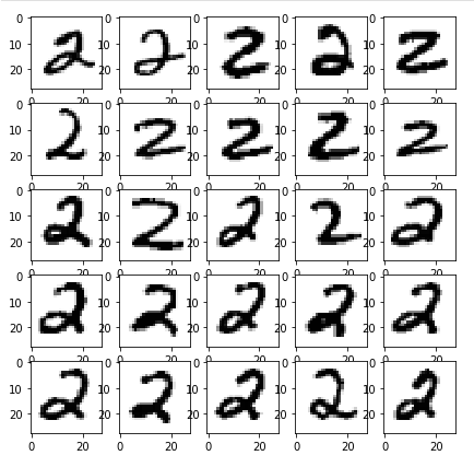
I “coincidentally” picked a great example! Completely unsupervised, K-means has done an amazing job in clustering all number 2’s together. Highly impressive, since we never even told it what the images contain. Sadly, it doesn’t cluster most other numbers this well. Let’s see it get confused by the similar curves of 8 and 3:
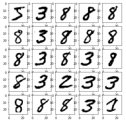
It especially struggles when dealing with the numbers which have a straight line, like 4,7,9. The following shows three classes which it matched to very similar data.
Insight
Here’s something cool. The centroids exist in the same feature space as the input data, so we can print them just the same! Let’s see what each class looks like.
reshaped_centroids = tf.reshape(centroids, (clusters_n, 28, 28))
fig = plt.figure(figsize=(15,8))
ax = []

for i in range(clusters_n):
    ax.append(fig.add_subplot(2, 5, len(ax)+1))
    plt.imshow(tf.reshape(reshaped_centroids[i], (28,28)), cmap="gray_r")
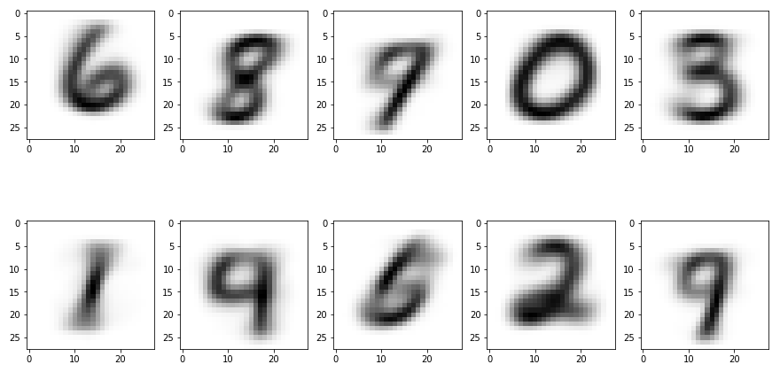
Looking at them it’s pretty clear what’s happening. While unique shapes such as 0, 1, and 2 were easy to separate, it really blurs the lines for similar ones. It clearly merges 8 and 3 together, and the 9 looks more like a 7 or a 4.
Since it operates on individual pixels, the algorithm has no clever way of grouping shapes and making sense of the data. Just like a simple dense layer it assigns weights to each pixel, but struggles with difficult decision surfaces.
Purity
A popular metric to measure clustering performance is purity. It measures how much of a single class is present in each cluster. A purity of 1 means that each cluster contains a single class. Let’s implement it for future reference.
def calc_purity(labels, assignments):
    # initialise a square matrix of size clusters_n with zeros
    # in it we'll keep track of the true label distribution per cluster
    d = np.zeros((clusters_n, clusters_n), dtype="int32")
    for l, a in zip(labels, assignments):
        # increase the number of label l assigned to cluster a
        d[a][l] += 1

    # divide highest label count per cluster by the total number of points assigned to it
    # the final score is the mean over all clusters
    return np.mean(d.max(1)/d.sum(1))

purity = calc_purity(y_train, assignments)
print(purity)
0.6256766873889321
conclusion
Hopefully, this post managed to show a simple way of applying the K-means clustering algorithm on the MNIST dataset. If your dataset has a low dimensionality and can be more easily linearly separated, this would be enough for your needs. In the next posts in this series, I hope to investigate methods of dimensionality reduction in order to improve our results.